Variational Filtering, Rebuilt From the Linear Case
A scalar linear-Gaussian benchmark made the VBF edge-factor implementation auditable before moving to nonlinear filtering.
Series: VBF Experiments, April 2026
Contents
This week started by rebuilding the variational Bayesian filtering experiments around a scalar linear-Gaussian state-space model. The goal was not to win on a toy problem. The goal was to make the mechanics testable before asking nonlinear questions:
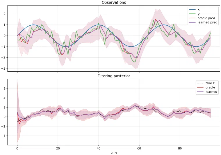
\[ z_t = z_{t-1} + w_t,\quad w_t \sim \mathcal{N}(0, Q) \]\[ y_t = x_t z_t + v_t,\quad v_t \sim \mathcal{N}(0, R) \]The filter carried a strict online marginal \(q^F_t(z_t)\) plus an edge/backward conditional \(q^B_t(z_{t-1} \mid z_t)\). That made the posterior edge factor explicit:
\[ q^E_t(z_t,z_{t-1}) = q^F_t(z_t)q^B_t(z_{t-1} \mid z_t) \]The immediate implementation work created JAX training and evaluation paths, analytic Kalman references, posterior diagnostics, predictive metrics, and plotting under src/vbf/, scripts/, and experiments/linear_gaussian/.
What Had To Be True#
The linear-Gaussian benchmark gave us closed-form answers. That allowed several checks which are hard to get in the nonlinear case:
- exact Kalman filtering should reach 90 percent coverage near
0.90; - a frozen marginal control should preserve the exact filtering marginal while learning only the backward edge;
- supervised edge heads should not be mistaken for an unsupervised result;
- Monte Carlo ELBO variants should be separated from oracle-calibrated diagnostics.
The frozen marginal control was especially important. It showed that the edge/backward conditional could be learned while the filtering marginal remained exact. In the five-seed diagnostic baseline, the frozen marginal row had state NLL 0.401983, coverage 0.900220, and variance ratio 1.000006, matching the exact Kalman marginal.
What The Sweeps Found#
The scalar report split results into weak-observability and randomized \(Q/R\) regimes.
| Regime | Strong reference | Learned row | Main result |
|---|---|---|---|
| nominal sinusoidal \(x_t\) | exact Kalman state NLL 0.402 | self-fed supervised state NLL 0.415 | supervised residualized filter was close |
| weak sinusoidal | exact Kalman state NLL 1.175 | MC ELBO state NLL 1.291 | unsupervised MC ELBO was under-dispersed |
| zero unobservable | exact Kalman state NLL 2.740 | MC ELBO state NLL 7.010 | local ELBO collapsed variance badly |
| randomized \(Q/R\) | frozen marginal matched Kalman | regime-local supervised was near reference | generalization needed explicit regime calibration |
The most useful negative result was that direct non-residualized ELBO training was weak. The strong rows depended on preserving analytic structure: residualized updates, frozen exact marginal controls, or oracle/reference calibration. That shaped the later nonlinear work: when results were good, the report had to say whether they were fully unsupervised or assisted by reference information.
ELBO And Predictive Checks#
The MC ELBO ablation behaved smoothly in the scalar case. Increasing samples improved state NLL from 0.575477 at one sample and 1000 steps to 0.542554 at 32 samples and 1000 steps. It still did not match exact Kalman state NLL 0.401983.
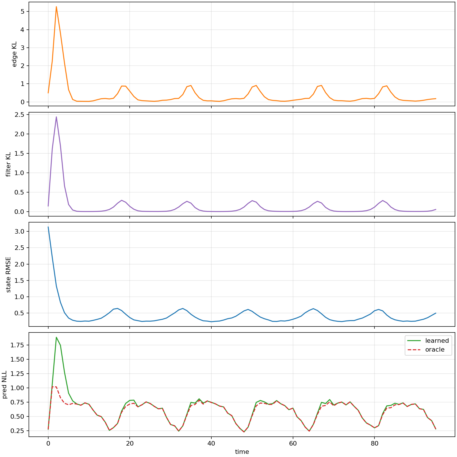
The predictive head experiment was a separate caution. With only short training it was poor, but at 3000 steps a learned predictive head on oracle belief reached predictive NLL 0.625870, close to exact Kalman predictive NLL 0.600858. A learned head on the ELBO belief reached 0.670554, while the analytic predictive from the same ELBO belief was 0.640331.
The interpretation was simple: the predictive machinery could be learned, but it was not a free substitute for a calibrated belief.
Why This Mattered#
The linear-Gaussian work made the later nonlinear reports stricter. The important labels were:
| Label | Meaning |
|---|---|
unsupervised | training used observations, known transition, known observation model, and prior |
reference_distilled | training used grid/reference moments, densities, or rollout targets |
oracle_calibrated | training used reference variance targets or oracle posterior statistics |
That labeling became the backbone of the nonlinear series. The scalar benchmark was ready once the report could say: self-fed supervised and frozen-marginal controls are useful diagnostics, but vanilla unsupervised ELBO remains under-dispersed in the regimes that matter.
Source artifacts: